The debate between allocating to a Value or a Growth fund is one that we come across all the time. Usually asset allocators are concerned that, at different points in the cycle, allocating to a Growth Fund may lead to underperformance which wouldn’t occur if they allocated to a Value Fund during that period. We would have hoped that this debate might have abated by now, but unfortunately it hasn’t.

In this article, we aim to go some way to resolving the aforementioned debate. In order to do this, we discuss Price and the specific models that have been developed to predict it. Secondly, we touch on Fundamental Value and its drivers. Finally, we will highlight why we don’t believe there should be any debate to begin with, and how if we reorient our thinking we can better outcomes for our clients.

Determining Price

Determining Asset Prices has been the subject of an enormous body of Academic research. The original Capital Asset Pricing model (CAPM) was proposed by William Sharpe in the 1960s. It proposed that the specific risk associated with an asset was the only driver of its price given systemic risks could be diversified away. In the 1970s Arbitrage Pricing Theory built upon these foundations and proposed that CAPMs specific risks could be broken into other more observable distinct variables, primarily macroeconomic, like interest rates and oil prices, to give you a more tangible driver of price. In 1992, Eugene Fama and Kenneth French published their 3 Factor Model (3FM) which showed that company specific factors like “Size” and “Value”, in addition to CAPMs Beta, were a better predictor of share price changes than CAPM was on it’s own. They determined this relationship through a least squares regression (Eqn 1).

The intuition behind the 3FM was that cheap stocks and smaller companies were more likely to provide better future returns than expensive or mature ones. We can see in Eqn 1 that the relationship to return of a security was clearly broken into four distinct parts: the market return, Small Minus Big (SMB,) High Minus Low (HML) and an error term (alpha).

The HML term is the measure of the “value” of a security, defined in terms of a Book/Price ratio — a high multiple was reflective of a cheap company and a low multiple reflective of an expensive company. SMB is a measure of the size of a company, defined as the inverse of the market cap — the smaller the number the less mature the company. The error term is the piece of the return that was unexplained by those other factors.

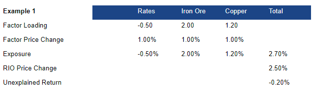
Below we illustrate how the pricing approach could be applied to determine the share price of Rio Tinto Limited (ASX: RIO) given some variables. In the example, RIOs price is negatively correlated to changes in interest rates (negative factor loading) and positively correlated with changes to the iron ore and copper (positive factor loadings). Iron ore being the biggest driver of the overall price change.

As each of the factors change, the price of RIO would change in proportion to the exposure it had to each of those factors. The unexplained portion of the return is the difference between the actual return and the return predicted by the regression analysis.

In our second example we illustrate how the 3FM can be applied to explain the return of a less mature, growing company like Megaport Ltd (ASX: MP1). In our example the return is negatively correlated with Value factors like book/price (so it’s deemed expensive). It is negatively correlated with Size (so it’s a Small Cap company) and is positively correlated with market movements. However, there remains a significant portion of the return that is unexplained by these factors.

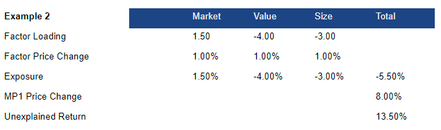
The key takeaway from these examples is that while these statistical factors can help predict a portion of the price movement in a related asset, there is a piece of the return that is not explained by these variables.

Understanding Value

Unlike pricing models, valuation models proposed by Academics tend to focus on things that are intrinsic to the businesses that they are trying to price. It is important to remember that these models are only representations of reality and have their limitations; however they are useful as they illustrate how changes to certain inputs impact the overall value of an asset.

For the purpose of explaining Value, we start with the Dividend Growth Model (DGM). The DGM (Eqn 2) states that the value of a company is the present value of the future distributable cash flows (CF), discounted by the spread between the cost of capital (k) and the expected growth (g) of those cash flows.

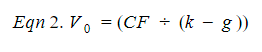
Distributable Cash Flows (CF) are defined as the amount left over after tax and investment to pay claimholders. The required rate of return, or the Cost of Capital (k), is the return required to compensate for the risk of investing in the company. Growth (g) is the increase that we could reasonably expect in those cash flows into the future.

Turning to Growth, it stands to reason that it requires investment and has natural limits. To get some sensible numbers we can assume that cash flows are able to grow by the return received (R) on the reinvested portion of the earnings. The choice we have to make then is how much of our earnings (E) are retained (b) and how much is paid out to claimholders as cash flow. We model these two ideas out in Eqn 3 and 4.

Combining these equations together we get our valuation model (Eqn 5). It takes into account an estimate of the earnings (E) the company will generate, the amount reinvested (1-b) and the expected return on that investment (R) and our expected return (k) (Eqn 5).

In Example 3, we assume that a company generates earnings of $10. For return on investment, we’ve used two scenarios, one where it is able to reinvest earnings at a return of 10% the other, where it gets a negative 10% return on investment. Our cost of capital is 5%.

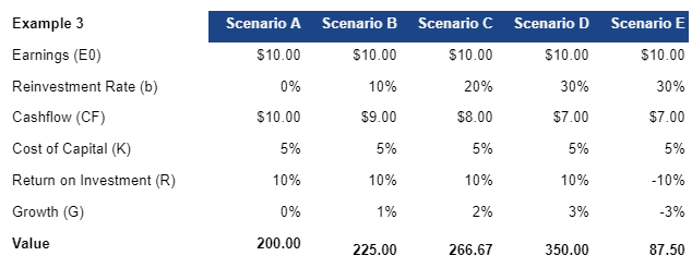
Given our example, we can make some observations. Firstly, as the reinvestment amount increases, so does the earnings growth rate (with one exception, Scenario E). In Scenario A, as no earnings are reinvested the value of the business is essentially the distributable earnings capitalised at your expected return, or $200.00 ([($10 * (1- 0%))/ (5%- (-3%))] through Eqn 1). Secondly, as we increase the reinvestment rate, the value of the business peaks at $350.00 (Scenario D), because we’re earning a return that is greater than our cost of capital. Finally, in Scenario E, despite a high reinvestment rate, the value of the business declines relative to Scenario A, because it earns a return that is below our cost of capital, thereby destroying Value.

The key observation here is that Growth and Value are linked. Said more simply: if for every dollar you spend, you only earn a dollar back, it doesn’t matter how much you scale, the business value doesn’t change. If you earn less than what you spend to generate those earnings, you go out of business reasonably quickly, and if you earn a profit on each dollar you spend you should invest more heavily.

So, where’s the debate?

In practice, the larger investment programs build their portfolios out in a similar fashion to the approach described to price assets. For example, they may have some broader market exposure, exposure to systematic factor premia (i.e. Growth, Value and Momentum) and hopefully some exposure to idiosyncratic returns through specialist managers. We usually run into the debate when asset owners are trying to pick the specialist managers for their idiosyncratic portion. The irony is that they look for a value manager, a small cap manager, a growth manager and so on.

Labelling a manager as a Small Cap, Growth or Value manager only makes sense when they are generating returns primarily through factor premia (remember the pricing models?). If that is true, then appointing them for that reason implies that Asset Owners are doubling up on the exposures that they should already be harvesting through other cheaper, more efficient quant strategies that focus on factor premia. If a manager is delivering primarily skill based, idiosyncratic alpha (remember the error term?) then labelling them as above is inappropriate as their returns are not driven by changes in prevailing factor exposures. The manager who generates primarily idiosyncratic returns, and can demonstrate a repeatable skill in doing so, should be the one that you appoint to manage the idiosyncratic portion of your program.

Hopefully we’ve illustrated that the Value vs Growth funds debate, shouldn’t actually be a debate at all. Actually, the debate is more driven by the fact that we’re using common terms to talk about different things. Where, the conversation should be more of a question about which managers are appointed to do which jobs in your portfolio program, and why.